Reviewing some key notes regarding the statistics.
probability distribution
When we discuss the concept about the probability distribution, what are we talking about? For discrete random variable, we just discsuss that table, for each value of that random variable, what are probability to select that value. The sum of values for all cases is 1.
For continuous variable, we mean that density function, the x axis is the value of variable. The y axis is just represent the density. The integration from negative infinity to positive infinity of x axis is 1. It is possible that the density value is larger or smaller than 1, there is no guarantee for that thing (do not mix this with the probability), only the integration of the density funcion can be the probability
Likelihood vs Probability
When discussing the pure defination of likelihood, just follow the documentation here. Likelihood is a strange concept in that it is not a probability but is proportional to a probability.
The likelihood of a hypothesis (H) given some data (D) is the probability of obtaining D given that H is true multiplied by an arbitrary positive constant K: L(H) = K × P(D|H). In most cases, a hypothesis represents a value of a parameter in a statistical model, such as the mean of a normal distribution. Because a likelihood is not actually a probability, it does not obey various rules of probability; for example, likelihoods need not sum to 1.
It takes me some time to consider why the L is proportinal to the P(D|H). For example, assuming there is gaussian cdf function, and the x axis is the variable, y axis is is probability densify value. For the likelihood function, its x axis can be some unknown parameter such as u, which is one parameter of the model in gaussian distribution. It is easy to get that the y value of the L function has a similar shape with the pdf. Assuming the data are knonw, we can get an prediction of u1 for its distribution, when value of u is far from the u1, associated y value is small, when u is close to the u1, associated y value is large, the shape of the L function is therefore quite similar to the shape of the pdf.
Pay attention, even for the conditional probability, it is still have a D and H notation. It might not be good to explain D and H in p(D|H) as event H and event D, it is good to explain it as data and hypothesis (a value of parameter in a specific distribution model). Key to distinguish them is to explain which one is fixed
Just remember that the likelihood is not the probability since the integration of the likelihood function is not nacessarily equals to 1.
In the context of the Bayesian ingerence, the P(D|H) is called the likelihood direaclty, its name only makes sense in the context of Bayesian, it is actually a pdf, not the formal defination of likelihood function.
Bayesan inference
When discsussing the Bayesan things, the defination of likelihood is a little bit different, the best explanation I can find is this one (https://www.youtube.com/watch?v=HZGCoVF3YvM&t=629s) at around 7:00. using the geographic representation to explain the Bayesan things can make it easier to understand. Pay attention that in the context of the Bayesan, the explanation of likelihood is a little bit different with the pure defination of the likelihood function. When we defien the likelihood function, we tend to use the L instead of the p. The L(theta) is not probability since the integration of the L is not necessarily 1. There are still some confusion about likelihhod for me. The easiest way is just to put them into different contexts. In the Bayesian context, just look at the grpahic representation, in the context with more strict defination, just use its pure defination.
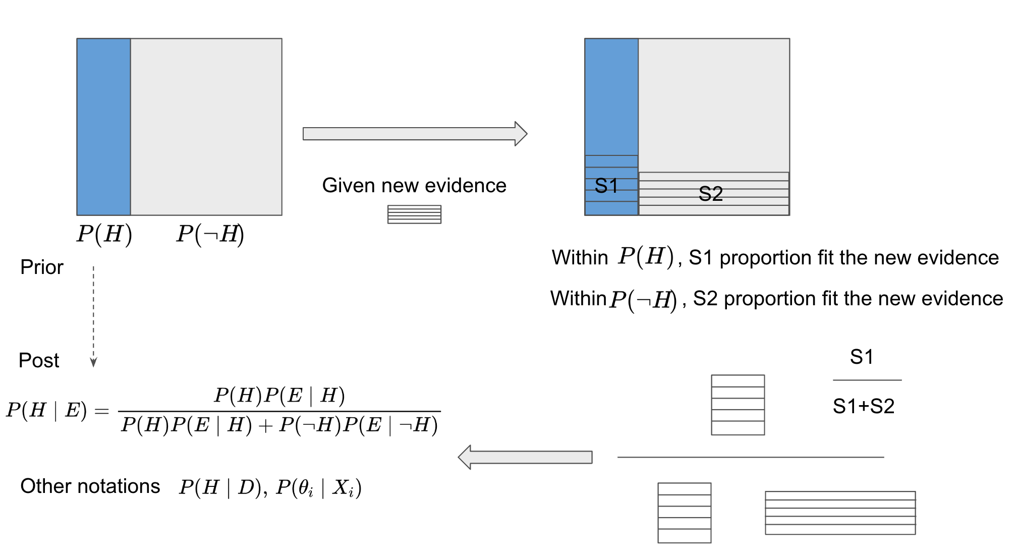
This figure shows a comprehensive understanding about the Bayesian Inference. The idea come from here, which is a really good video to explain associated ideas from graphic view. Instead of memorizing the equation, it is more convenient to memory the graphical figure to show the main idea. The main idea is to update the belief of the probability based on new evidence (data), as the explanation in the video, the evidence or the new data is just the thing that helps to update the belief instead of determine it. After understanding this figure, we can easily utilize the Bayesian inference into different contexts.
Covariance matrix
This blog provides a good example for computing the covariance matrix from scratch. The output of the covariance matrix computation is a matrix, and each element is a cov value. The i,j position of this matrix is cov(xi,xj). The key is to understand how to compute the cov(xi,xj). Assuming the sample of one attribute is (x1,x2…xn) another attribute is (y1,y2…yn). The first step is to compute the mean value of x and y, namely, MeanX and MeanY. Then we can get a new attribute value for each sample, (x1-MeanX)(y1-MeanY), (x2-MeanX)(y2-MeanY)…(xn-MeanX)(yn-MeanY). Then we can compute the mean value of these new matrix, this is the cov(X,Y) value. The covariance of the two attribute, each attribute can contain multiple samples.
Assuming there are two attribute, the original matrix is
then we can compute the average value of each attribute, and get a new matrix
after that, we can get the covariance matrix by , for each element, there is
Histogram and Kernel density estimation
Currently, we put all these information into another blog that discussed the MG and GMM
大数定理 中心极限定理
期望 方差 协方差
面试问题 随机变量x的期望是2,那x平方的期望是多少